Overview
The i.LON® SmartServer from Echelon® provides a useful data logging feature. The resulting log can be stored in XML or CSV (comma separated varible) formats. This article describes post-processing the CSV format within Microsoft Excel®.
Date/Time Format
The SmartServer stores the date and time in a format like:
2010-06-28T18:15:00.060-07:00
Excel does not recognize this format unless you make some changes:
- Replace the timezone indicator “-07:00” with nothing. Use the “Find and Replace” dialog and put “-07:00” or whatever your timezone value is into the “Find what:” box. Then clear out the “Replace with:” box and click “Replace All”.
- Replace the “T” between the date and time with a space. You can do a global search and replace of “T” with ” “, but this will mess up other places that “T” (or “t” if you don’t select “Match case”) appears. To prevent this, you can do three find and replace steps:
- Replace “T0” with “T ” (use “Match case”).
- Replace “T1” with “T ” (use “Match case”).
- Replace “T2” with “T ” (use “Match case”).
- As you replace the “T”s, you will probably see the dates change into numbers or times (without a date). To fix this, do the following:
- Select the entire “A” column, right-click and select “Format Cells…”.
- Set the “Number” category to “Time” and select one of the last two entries on the list “3/14/01 1:30 PM” or “3/14/01 13:30”.
- If you want to add the seconds, then select the “Custom” category and edit the “Type:” box to show “m/d/yy h:mm:ss;@”.
UCPTpointName
The point names are all prefixed with a long path. If you don’t need this path, it’s more convenient for the following steps, if you remove it.
- Click on one of the point names and select everything up to and including the last slash. For example:
- Building One/Channel 1/iLON SmartServer/Web Server- 0/
- Load the “Find and Replace” dialog and replace this path with nothing.
Unused Columns
In our experience, the following columns are not used and can be deleted:
- UCPTalias
- Reserved
- UCPTpointStatus
- UCPTvalueDef
- UCPTpriority
Sorting the Data
The log on the SmartServer can be configured for circular operation, meaning it will wrap around and start overwriting old data. This means the log records may not be in order. To fix this, we recommend selecting all columns, then use “Data – Sort” to sort the data, generally by the “UCPTlogTime” column. Depending on your application, you may want to sort in “Oldest to Newest” or “Newest to Oldest” order.
Filtering the Data
If you select “Data – Filter”, Excel will add dropdown arrow boxes by each heading in the top row. We use this so that we can filter on a single “UCPTpointName”, such as “nviDemand”.
Once you’ve filtered on a data point, you can then select the filtered cells, copy and paste them to a new worksheet, and then chart or analyze them easily.
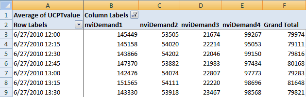
PivotTable
Excel has an advanced feature called a “PivotTable”, which is very useful for analyzing large sets of data with multiple data points for each log time. The PivotTable allows you to arrange the data so that each date/time value has one row and each UCPTpointName has one column. This way, you can see all the data points for a particular time in one row, rather than spread out over many rows. This also makes it much easier to graph particular data points.
There are a few tricks to using the PivotTable.
Adjusting the Times
Suppose you are logging every fifteen minutes. The actual log times won’t all be exactly identical, but may vary by several seconds. This can cause the data from one 15 minute interval to get spread out over a few rows. To fix this, you need to create a new column to the right of “UCPTlogTime” that contains an adjusted time.
The following equation adjusts the time for fifteen minute intervals:
=ROUND(A2*24*60/15,0)/(24*60/15)
If you are using different time intervals, change the “15” which appears twice in the formula to the correct number of minutes. Paste this formula into all cells in the “B” column next to valid date/time values in the “A” column. Use “Format Cells…” to diaplsy the value as a well formatted date/time as described above.
Create the PivotTable
Now select the three columns with the adjusted time, UCPTpointName, and UCPTvalue. Use “Insert – PivotTable” to create a new PivotTable on a new worksheet. The PivotTable will appear on the left (initially empty) and the configuration screen on the right.
- Drag the adjusted time “Adj Time” field into the “Row Labels” box.
- Drag the “UCPTpointName” field into the “Column Labels” box.
- Drag the “UCPTvalue” field into the “Values” box.
Measure the Average
Depending on the data, Excel may choose to display the sum or count of the UCPTvalues. The “Sum” is acceptable, but it’s generally better to click on the field in the “Values” box, select “Value Field Settings…” and then choose “Average” from the list. That way, if for some reason, there are two data points for a single time interval, it will display the average value.
Using the PivotTable
Now that you have the PivotTable, you can easily graph different columns verses the log times.
If you want to manipulate the data further with formulas, you may need to select the entire PivotTable, copy it, then use “Paste Values” to paste it somewhere else. Then use formulas on this copy. Formulas don’t work as well on the original PivotTable, because they don’t use normal cell references.